Your First Design

This tutorial walks you through building a compliant mechanism from scratch, starting from an empty scene and finishing with a fully optimized topology. It takes about five minutes.

What you will build

You will design a compliant force redirector — a mechanism where pushing rightward on one corner causes the opposite corner to move downward. This demonstrates how the solver can create mechanisms that change the direction of force by 90 degrees.

The setup:

• A 100 mm x 100 mm rectangular plate
• An input force near the top-left pushing rightward
• A target output point near the bottom-right where motion should occur downward
• Two fixed supports that act as pivot points for the mechanism
• ABS plastic as the material
• A pair linking the input to the output with K_p_max tuned for ABS
• A volume fraction of 0.3 (keep 30% of the material)

The solver will produce a design with flexural members that route through the fixed supports, redirecting the input force 90 degrees at the output.

Let's build it.

---

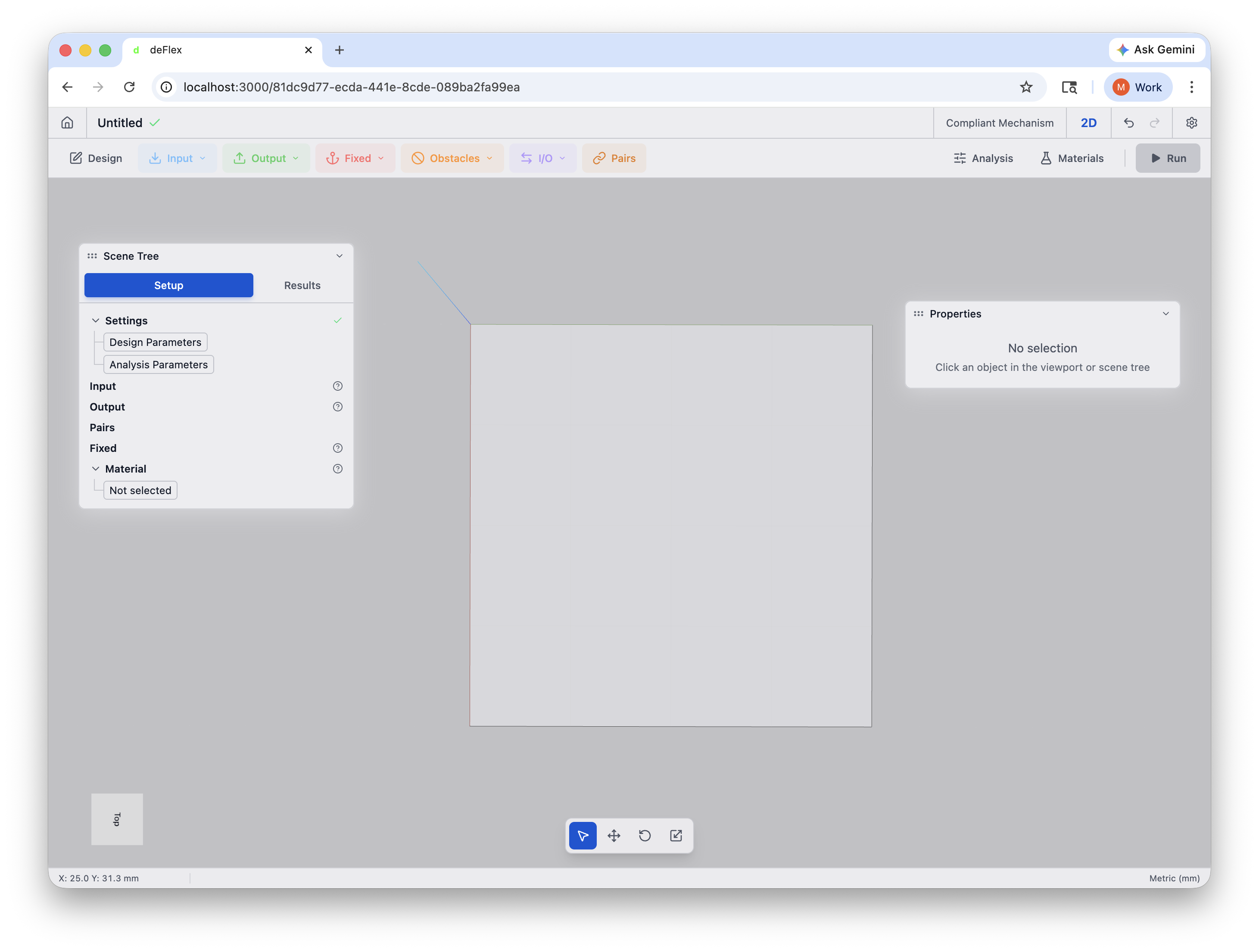
Step 1: Create a new scene

1. From the home page, click the + New button.
2. Select the Compliant Mechanism analysis type, then choose 2D.
3. The scene opens in the editor with a default design domain. To rename it, click the gear icon in the top-right corner, go to the Scene tab, and edit the name to "Force Redirector."

You now have an empty scene with the 3D viewport, scene tree, and properties panel visible.

---

Step 2: Add a design domain

The design domain defines the region where the solver can place material. For this tutorial, you will use a simple rectangular plate.

1. In the toolbar, click Design to open the Design Settings panel.
2. The scene was created with a default design domain. In the Design Settings panel, set:
   • Design Domain Width: 100 mm
   • Design Domain Height: 100 mm
   • Element Size: 1.0 mm (this produces a 100 x 100 grid with 10,000 elements -- fine enough for a clear result, fast enough to solve in under a minute)

note

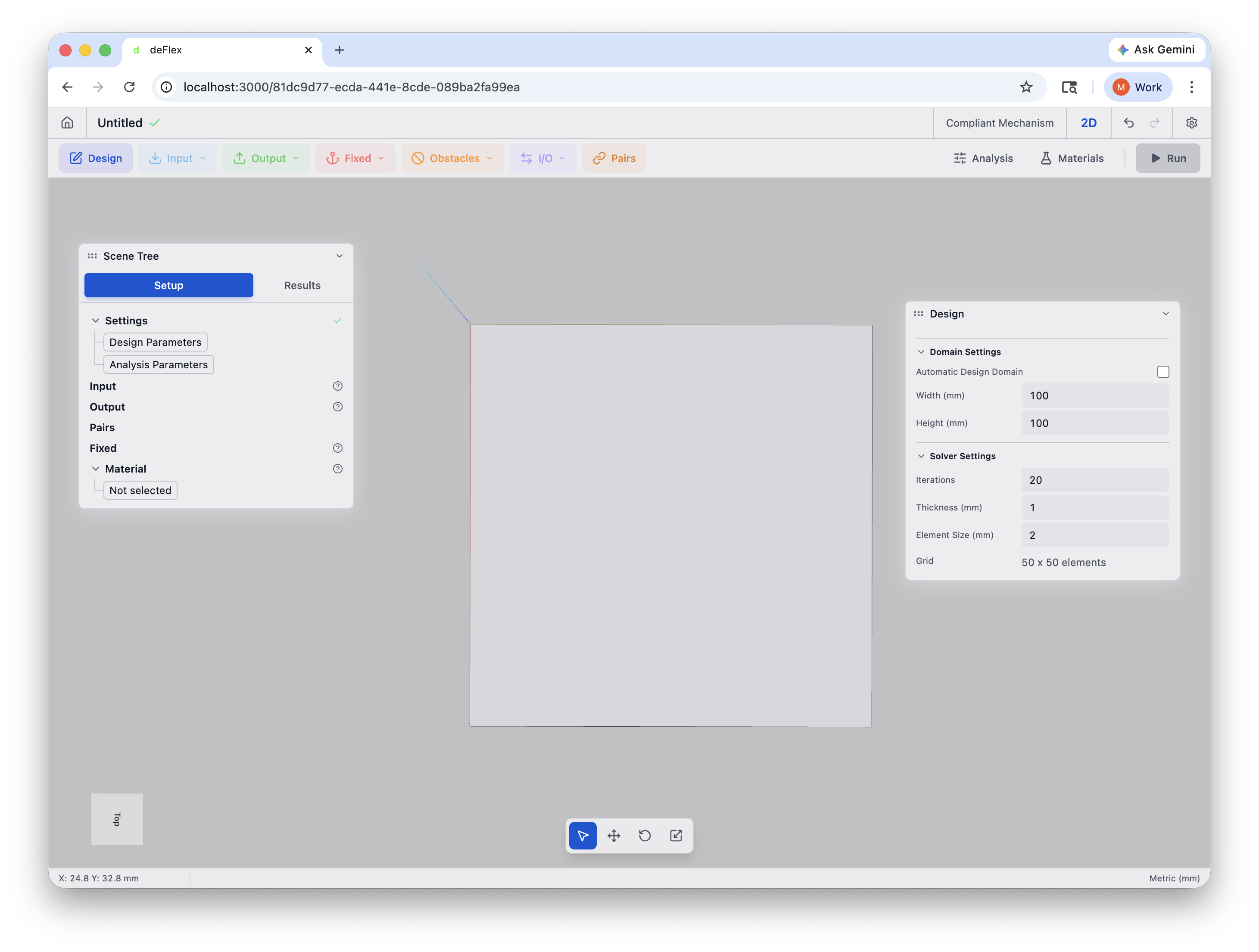
Element Size controls the fidelity of the optimization. Smaller elements produce finer features but take longer to solve. For this first tutorial, 1.0 mm on a 100 x 100 mm domain is a good balance between speed and quality.

---

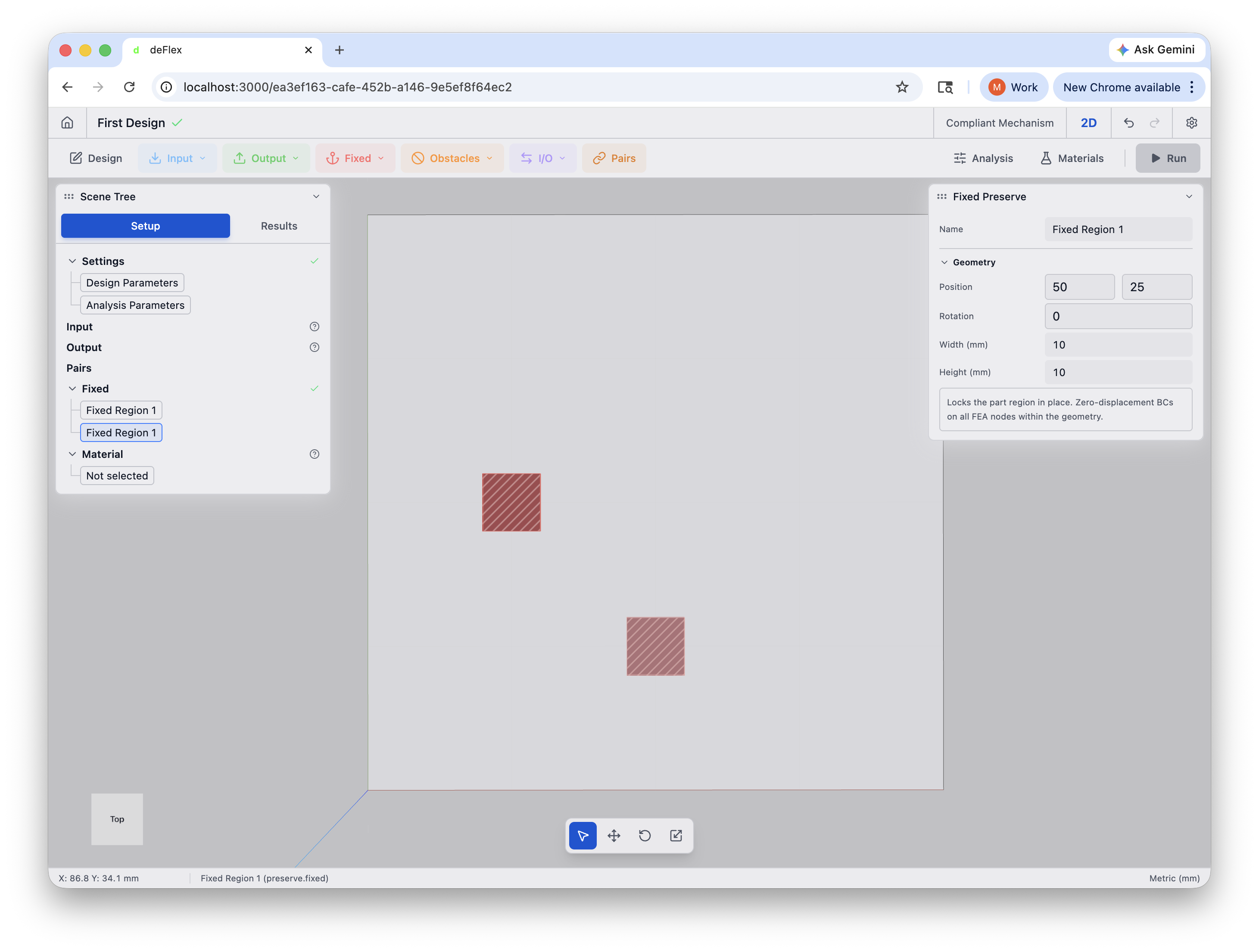
Step 3: Add fixed supports

The mechanism needs fixed supports to act as pivot points — without them, the structure would just slide freely. You will place two fixed regions between the input and output.

Add the first fixed support

1. In the toolbar, click the Boundaries dropdown and select Part-based.
2. A fixed preserve region appears on the plate. Select it.
3. In the properties panel, set:
   • Position X: 25 mm
   • Position Y: 50 mm
   • Width: 10 mm
   • Height: 10 mm
4. Right-click the preserve in the scene tree and select Rename to name it "Fixed -- Left Center."

Add the second fixed support

1. Click the Boundaries dropdown again and select Part-based.
2. Configure it:
   • Position X: 50 mm
   • Position Y: 25 mm
   • Width: 10 mm
   • Height: 10 mm
3. Right-click and rename it to "Fixed -- Bottom Center."

Both fixed supports now show preserve markers in the viewport, positioned between the input and output locations.

tip

Use scroll-wheel zoom and left-click drag to orbit, keeping the viewport centered on your work area as you add elements.

---

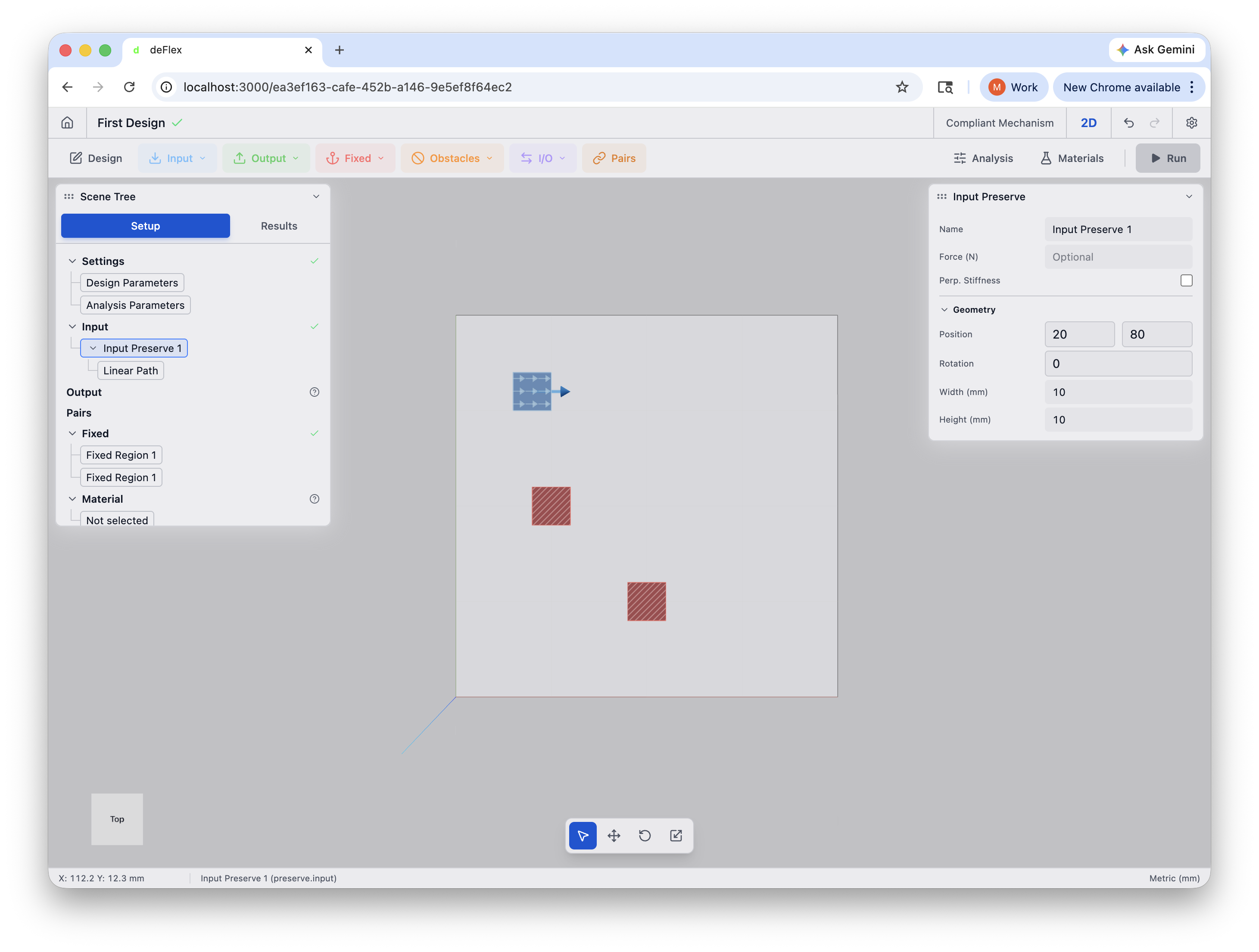
Step 4: Add the input force

The input force is where you push the mechanism. You place a small rectangular input pad near the top-left of the plate.

1. In the toolbar, click the Input dropdown and select Rectangle.
2. A new input preserve appears. Select it and configure:
   • Position X: 20 mm
   • Position Y: 80 mm
   • Width: 10 mm
   • Height: 10 mm
3. Right-click and rename it to "Input Pad."
4. With the input pad selected, look for the Boundary Condition section in the properties panel (or add a force boundary condition from the toolbar and attach it to this preserve).
5. Set:
   • Type: Force
   • Direction: +X (rightward)
   • Magnitude: 1.0 N

tip

Don't place preserves flush against the domain boundary. The solver needs material area around each preserve to generate connecting topology — if a preserve sits right at the edge, there is no room for the solver to create structure on that side. Leave a gap between preserves and the domain boundary. Alternatively, use Automatic Design Domain in the Design Settings panel, which calculates the domain size from your preserve positions and adds configurable padding (default 20%) so you don't have to manage spacing manually.

An arrow appears on the input pad in the viewport showing the direction of the applied force.

---

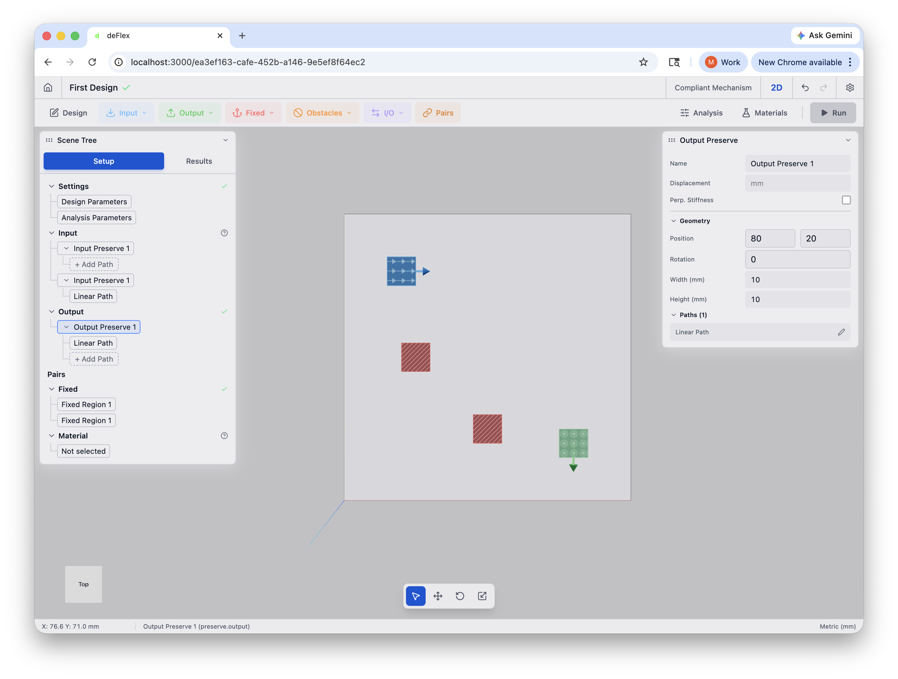
Step 5: Add the output target

The output target tells the solver where you want the mechanism to produce displacement. You place a small rectangular output pad near the bottom-right of the plate. The output should move downward — a 90-degree redirection from the rightward input force.

1. In the toolbar, click the Output dropdown and select Rectangle.
2. A new output preserve appears. Select it and configure:
   • Position X: 80 mm
   • Position Y: 20 mm
   • Width: 10 mm
   • Height: 10 mm
3. Right-click and rename it to "Output Pad."
4. Set the output direction to -Y (downward) in the properties panel.

The output pad now shows a direction marker in the viewport indicating where displacement is being measured.

---

Step 6: Create a pair

A pair links an input preserve to an output preserve and tells the solver which input drives which output. Each pair also carries a K_p_max (maximum characteristic stiffness) constraint that affects how the solver generates topology.

1. In the scene tree, click Pairs to expand the section.
2. Click + Add Pair (or use the Pairs button in the toolbar).
3. Assign the Input Pad as the input and the Output Pad as the output.
4. Set K_p_max to 2.0 N/mm.

note

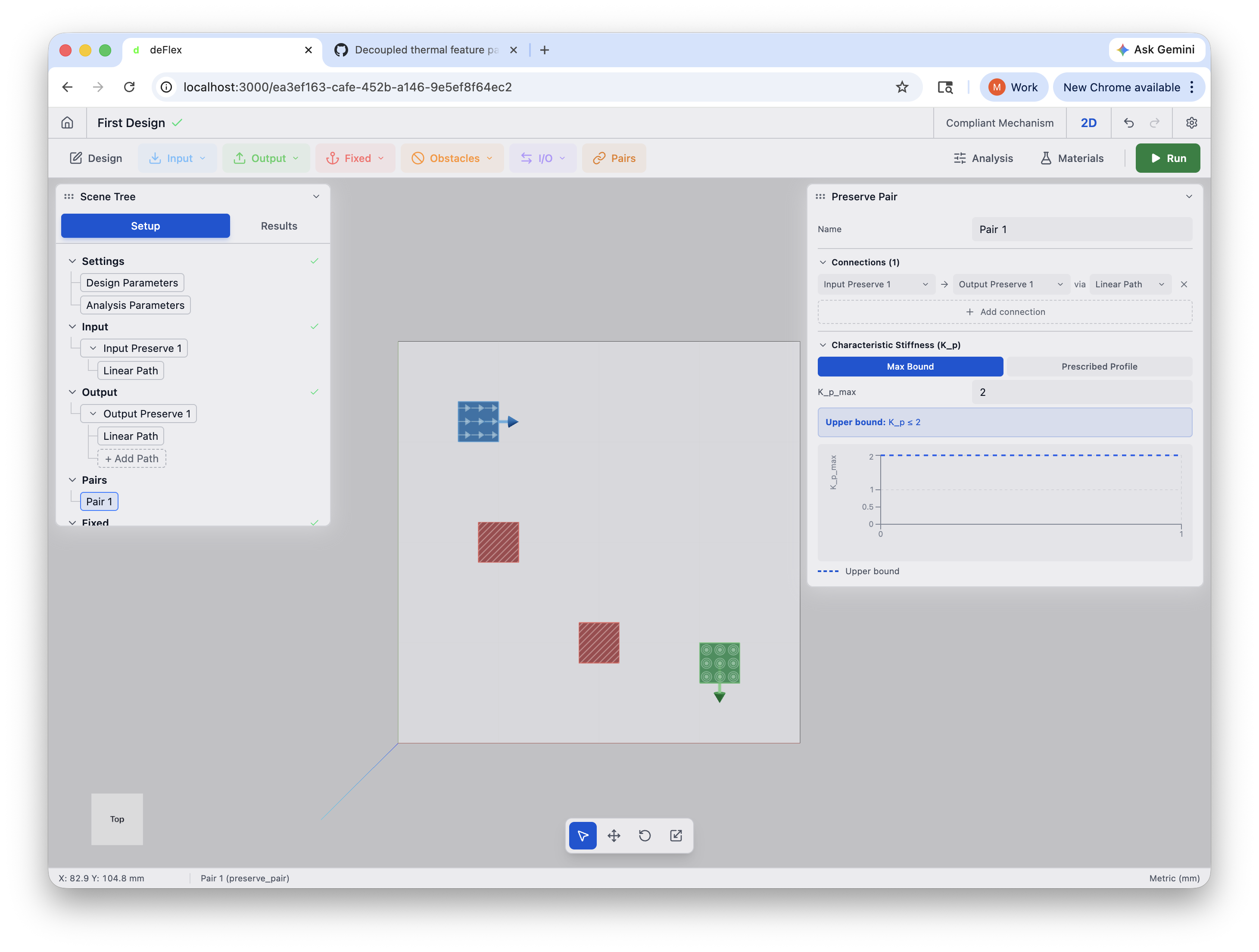
K_p_max controls how stiff the mechanism's output can be. The right value depends on your material — stiffer materials (like steel) can use higher values, while softer materials (like ABS plastic) need lower values. For ABS, a K_p_max around 2.0 is a good starting point. If the solver does not converge, try adjusting K_p_max up or down.

---

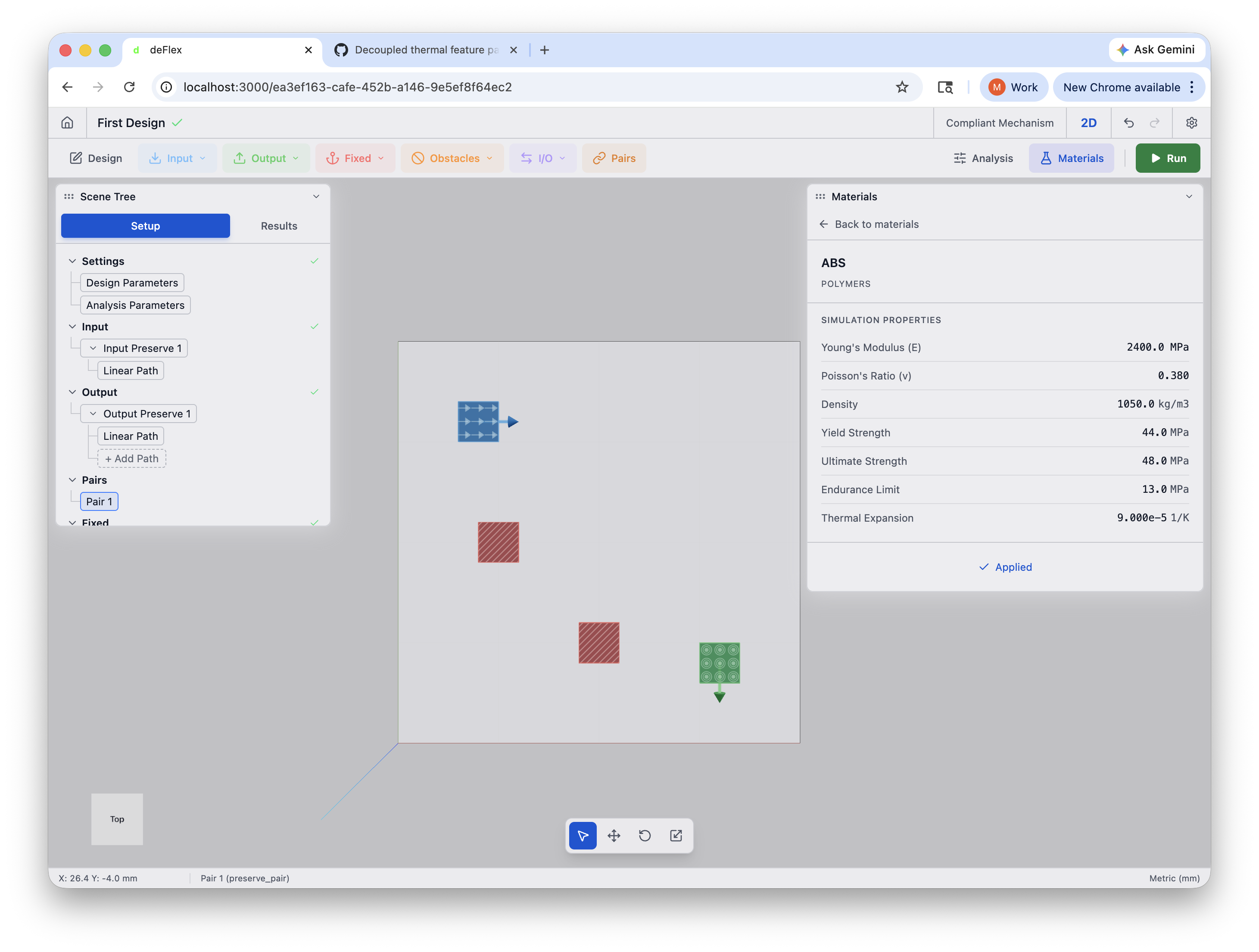
Step 7: Select a material

1. In the toolbar, click Materials.
2. Select ABS from the material list.

The material properties (Young's modulus, Poisson's ratio, density) update automatically. ABS is a common 3D-printing plastic and works well for compliant mechanism designs.

---

Step 8: Configure the solver

Now you need to tell the solver how to optimize.

1. Click Analysis in the toolbar to open Analysis Settings.
2. Set:
   • Volume fraction: 0.3 — the solver will use at most 30% of the design domain's volume. This forces the algorithm to find efficient load paths rather than filling everything with material.
   • Maximum iterations: 50 — the solver will run up to 50 optimization iterations. Most problems converge well before this limit.
   • Filter radius: 1.5 — this controls the minimum feature size and prevents numerical artifacts.

warning

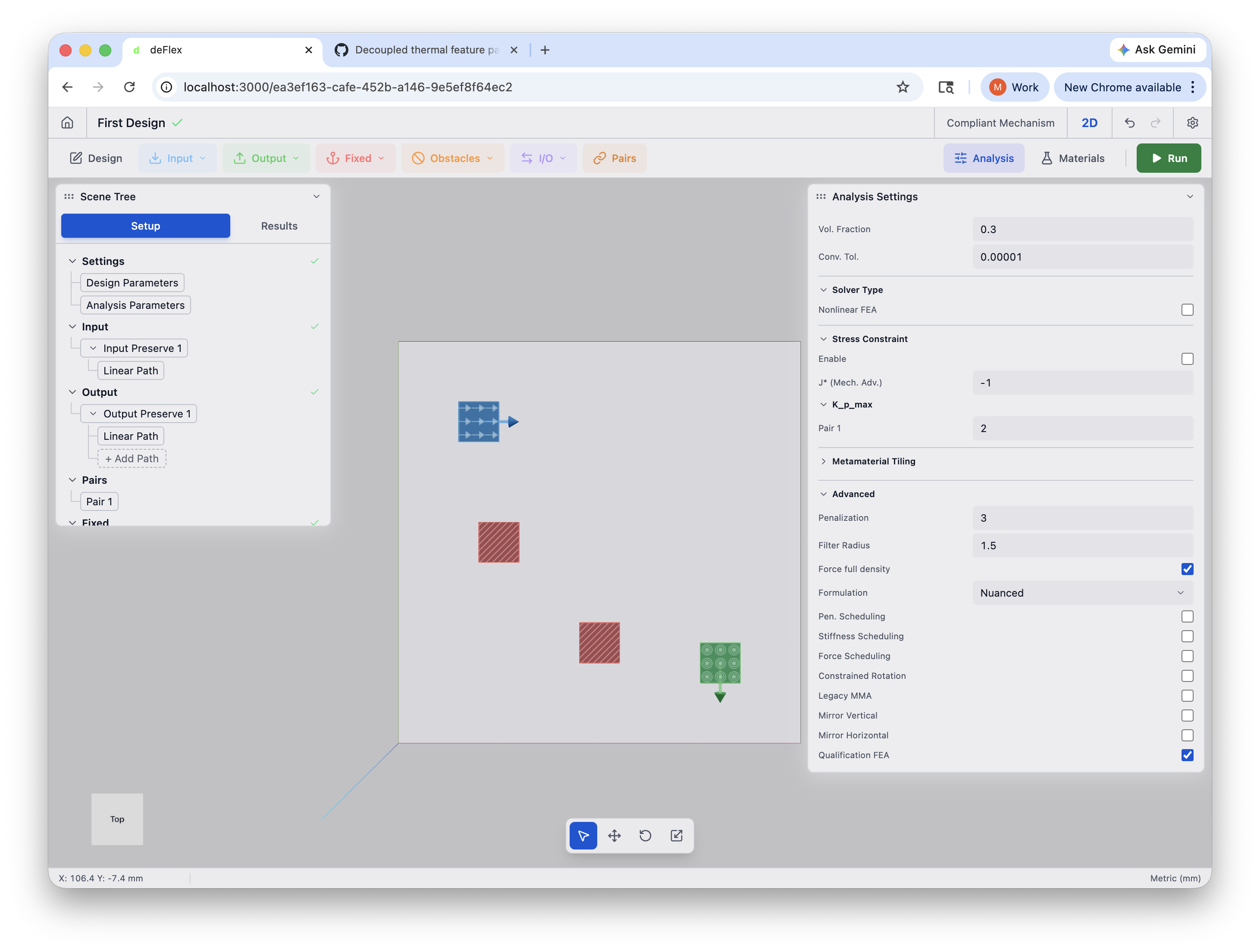
A volume fraction that is too low (under 0.15) may produce a design that is too sparse to be structurally viable. A volume fraction that is too high (above 0.6) may not produce interesting topology — the solver has too much material to work with and will not need to make hard choices about where to place it. For most problems, 0.2 to 0.4 is a productive range.

---

Step 9: Run the solver

Everything is set up. Time to let the solver work.

1. Click the Run button in the toolbar.
2. The solver run card appears in the sidebar showing progress. The iteration counter updates as the solver works.
3. Watch the viewport: the material layout updates live after each iteration. You will see the initial uniform gray field gradually resolve into distinct solid and void regions.

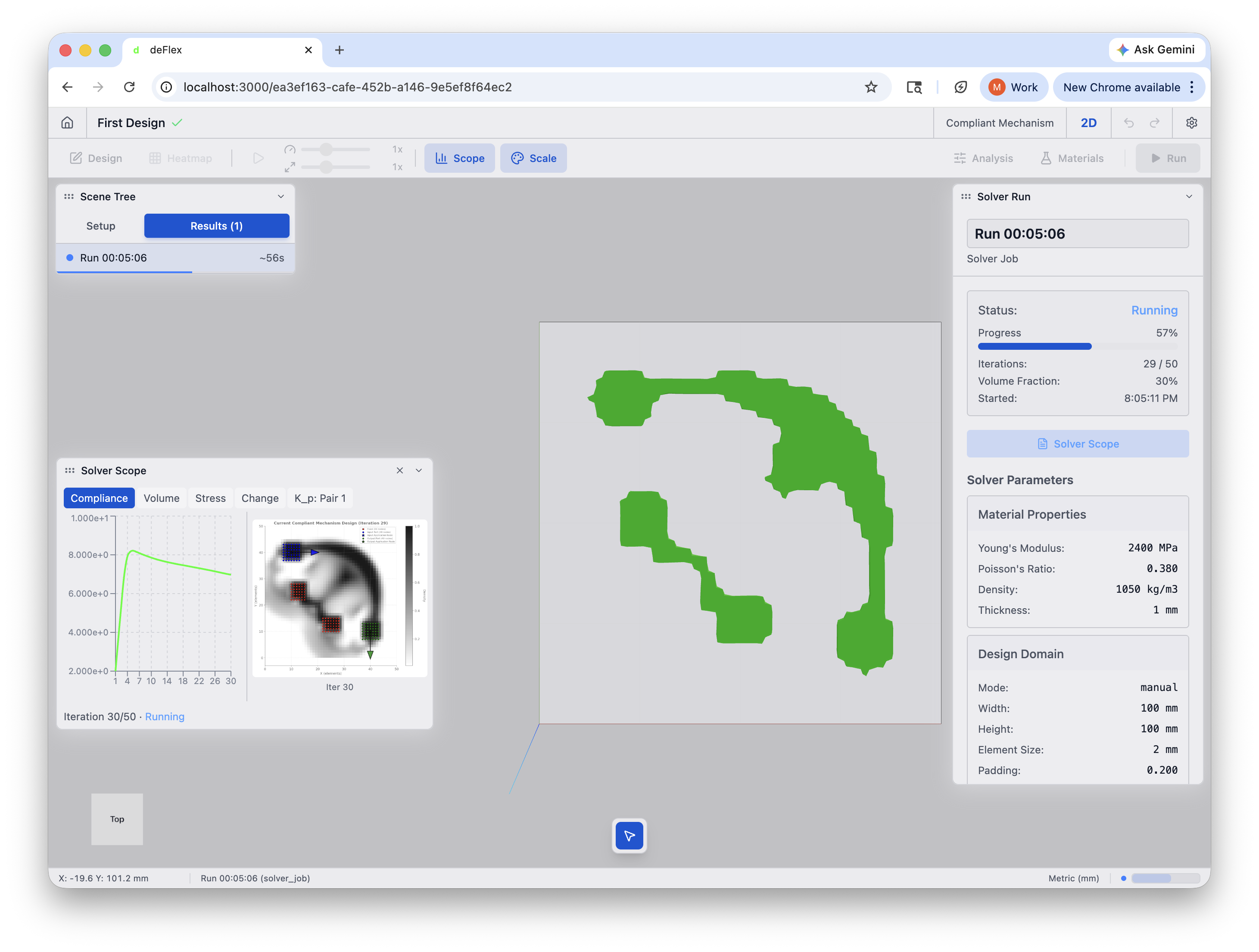
The solver typically converges in 30-50 iterations for this problem. You will see the design performance improve rapidly at first, then flatten as the design stabilizes. The algorithm automatically stops early if it detects convergence before reaching the maximum iteration count.

---

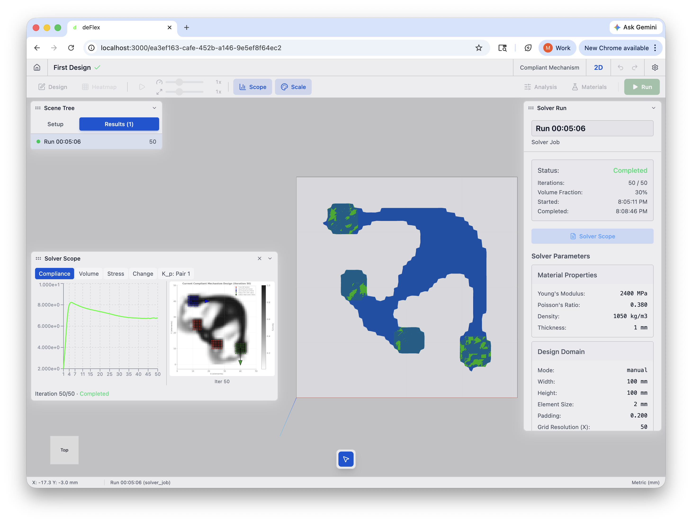
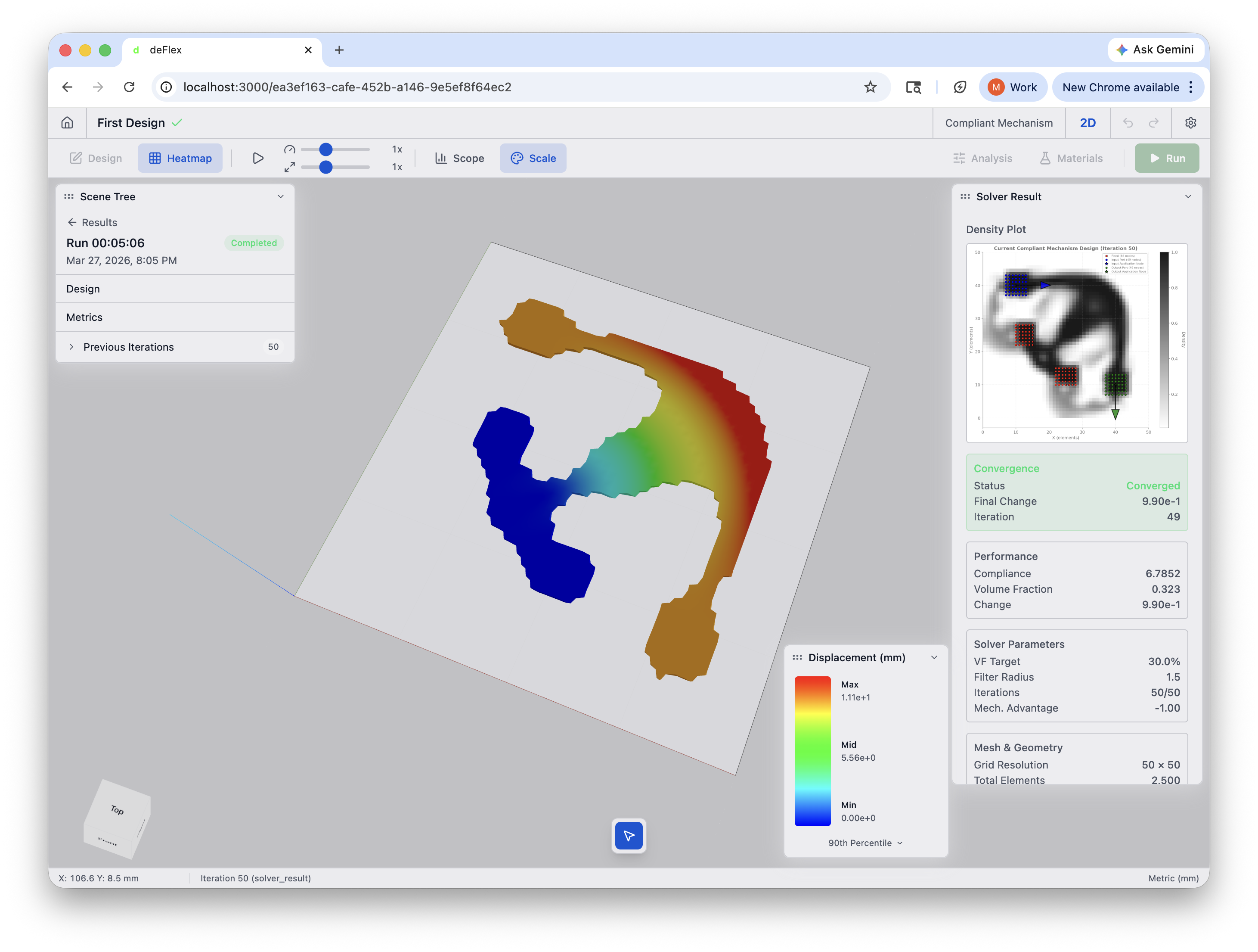
Step 10: Review the result

When the solver finishes, the run card shows a green "Completed" status. The viewport displays the final optimized design.

You should see a curved topology — flexural members routing from the input pad through the fixed supports to the output pad. The material forms an arc that redirects the rightward input force into downward motion at the output.

What to look for

• Clear solid/void separation — the material layout should have mostly solid (green) and void (empty) regions, with minimal intermediate material. A well-converged result has crisp boundaries.
• Connected load paths — trace the path from input to output. The material should form continuous members connecting the pads through the fixed supports. If the topology is disconnected, the problem setup may need adjustment.

Inspecting the convergence

Click the solver run in the Results tab to view convergence data. The right panel shows:

• Convergence status — whether the solver converged and the final change value.
• Compliance — the design performance value. Should decrease over iterations.
• Volume fraction — should match your target (0.3).

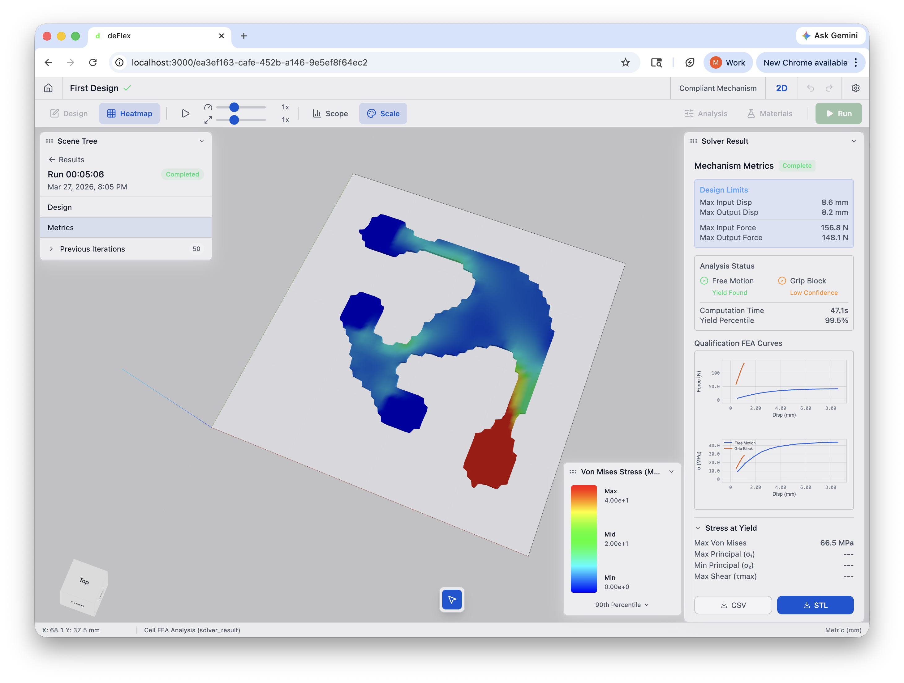
Post-solve analysis

After the solve completes, deFlex runs a qualification analysis on the result. Click Metrics in the left panel to see mechanism performance data including maximum displacement, forces, stress analysis, and yield percentile.

---

Step 11: Adjust and re-run (optional)

If you are not happy with the result, you can adjust parameters and re-run:

• Too sparse / disconnected? Increase the volume fraction (try 0.4).
• Features too thin? Increase the filter radius (try 3.0).
• Not converged? Try adjusting K_p_max — lower it if the solver oscillates, raise it if the result is too soft. Also try increasing maximum iterations (try 200).
• Want finer features? Decrease the Element Size (try 0.67 mm for a ~150 x 150 grid), but expect a longer solve time.

Each run starts fresh from a uniform material layout. Previous results do not affect subsequent runs.

---

What you learned

In this tutorial you:

1. Created a Compliant Mechanism 2D scene with a rectangular design domain
2. Placed preserve regions for fixed supports, an input pad, and an output pad
3. Applied a force boundary condition to the input
4. Specified an output displacement direction
5. Created a pair linking the input to the output and set K_p_max
6. Selected ABS as the material
7. Configured the solver with volume fraction, iteration count, and filter radius
8. Ran the design optimization and watched it converge
9. Reviewed the result for clear topology, convergence, and connectivity

This is the core workflow for every design in deFlex: define geometry, mark preserves, set boundary conditions, configure, solve, review.

---

What's next?

Now that you have the basics, explore these topics to deepen your understanding:

• Interface Overview — full details on every part of the UI, keyboard shortcuts, and viewport controls
• Understanding Preserves — learn about the different preserve roles and how they affect optimization
• Solver Settings Explained — detailed guide to every solver parameter and how it affects results
• Importing STEP Files — work with real CAD geometry instead of simple rectangles

tip

Experiment with different volume fractions, mesh resolutions, and boundary condition layouts. Design optimization is highly sensitive to problem setup, and exploring the design space is the best way to build intuition for what produces good results.